An OpenStereo Tutorial

First, install OpenStereo by following the instructions on the installation page for your operating system. Make sure to update whenever a new release is available.

After installing, open the program either from your start menu or from command line as either:

python -m openstereo

Or:

openstereo

Optionally, an .openstereo project file can be opened:

openstereo example_project.openstereo

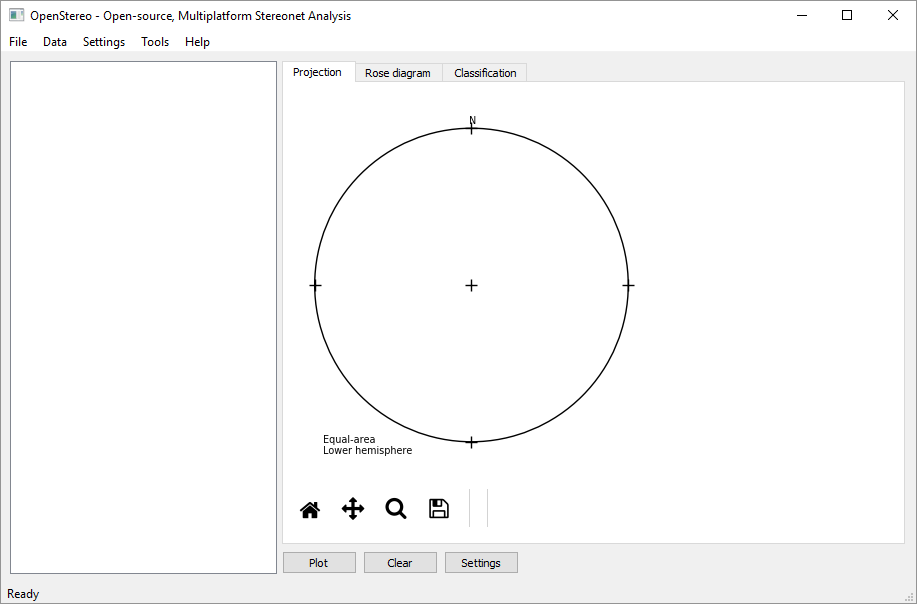
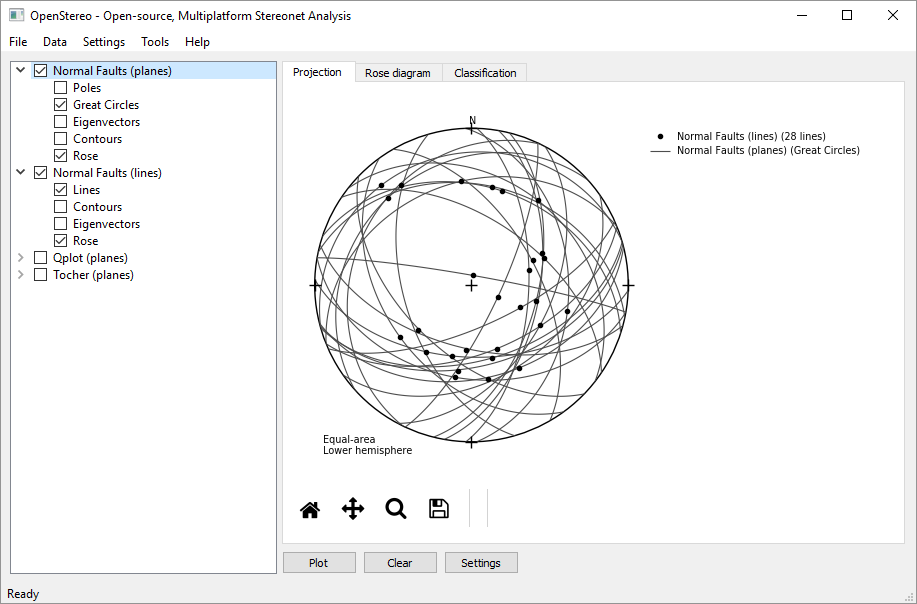
From that, you are brought to the main window:

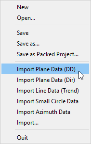
From the File menu you can open or save projects and import files. The quickest way to open a simple data file is using the specific import actions. for example, Import Plane Data (DD):

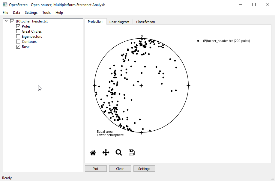
OpenStereo supports both CSV files and excel spreadsheets. Download tocher_header.txt from the example data directory inside the repository and select it after clicking this option. After loading, either click Plot or press Ctrl+P on your keyboard to view the poles of this example:

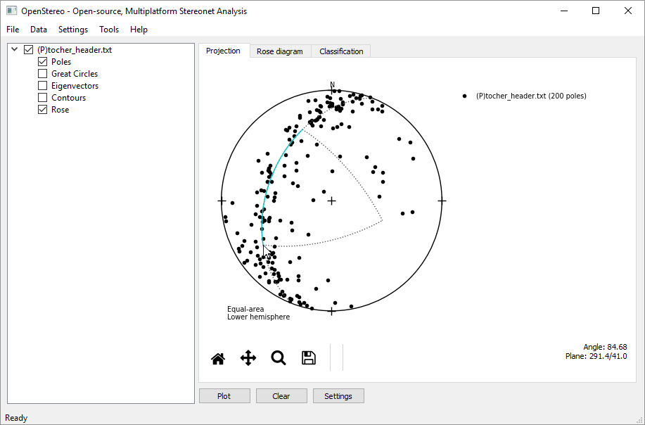
The Projection plot is interactive. The attitude of the point under the mouse will appear on the lower right corner when you mouse over the plot. Also, if you click and drag over the plot you’ll be able to both measure angles and see the attitude of the plane formed by the point you first clicked and the current point:

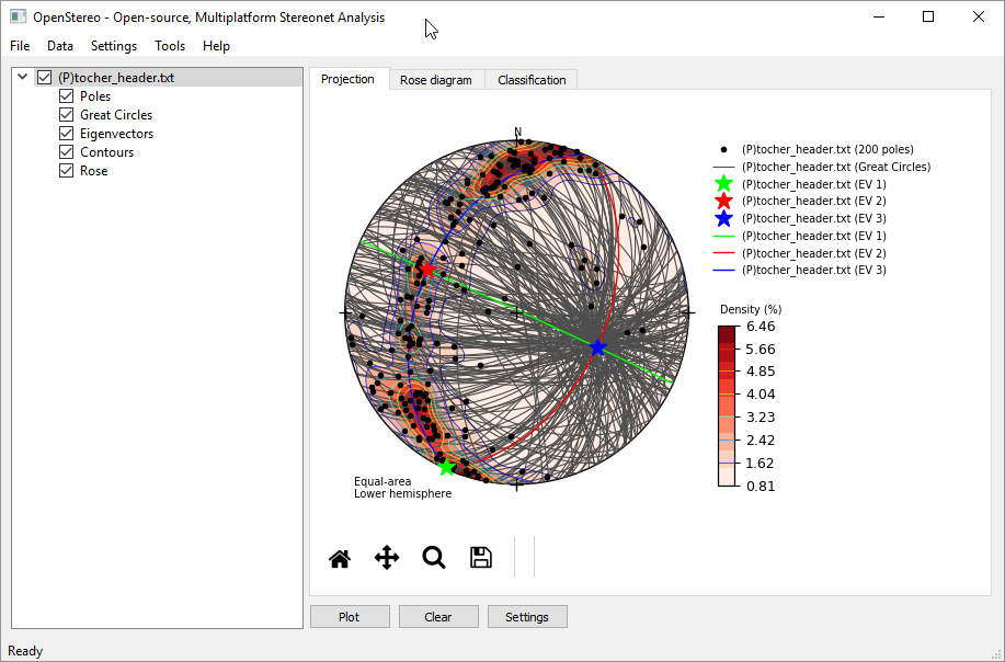
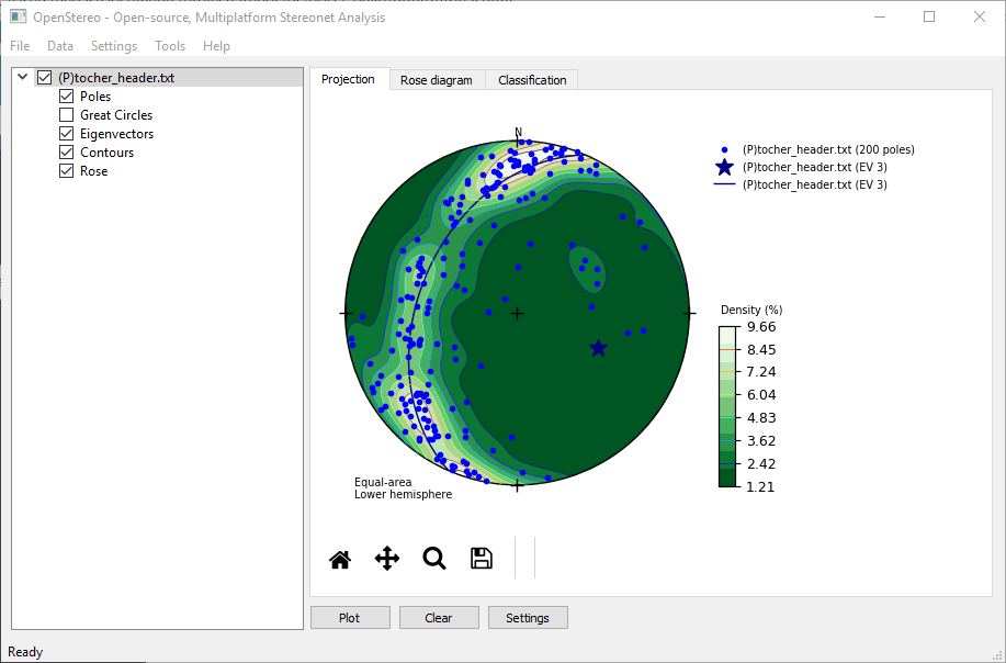
It is also possible to plot the great circles, eigenvectors and contours of a planar dataset. Click on the check boxes of these options under the (P)tocher_header.txt item on the data tree and press plot to get a very busy view of the data:

Disable the Great Circles option for now and right click on the Tocher item (or over any of its options) to get its context menu:

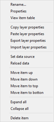
You can rename, delete, reorder, reload and change the display properties of the item using this menu. Click on Properties to do so:

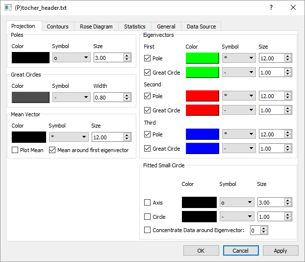
Most plot options for the Projection plot tab on the main window are located on this first tab, with the exception of contour plots. Try changing some options, such as color and size of poles (on the top left), while disabling poles and great circles of the first and second eigenvectors, and change the color of the pole and great circle of the third eigenvector. If you click OK the changes will be accepted and the dialog will close, but if you click Apply instead, the dialog will remain open.

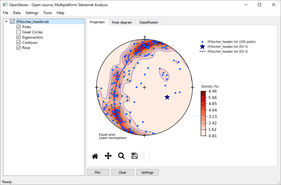
You can keep the dialog open and still interact with OpenStereo, even while opening the properties dialog of multiple items. Press apply and see the changes on the plot:

On the Contours tab of the properties dialog you may change the many different related options:

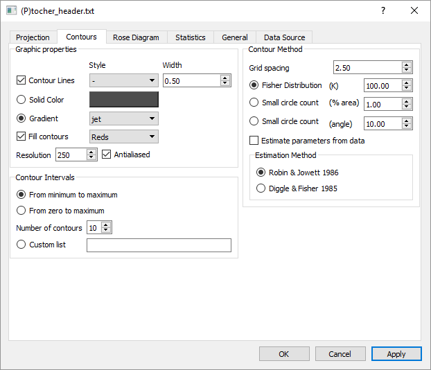
Try a few different graphic options for the contours, as changing the fill contours gradient to something like Greens_r. You may also change the number of contours and the way they are built. In the right side, it is possible to configure which method will be used for the contouring, either as a count of the number of poles inside a small circle around each node or by exponentially smoothing each point to every node using the Fisher distribution.

The parameter K controls how smooth the contribution of each point will be. Smaller values of K will smooth more, while larger ones will make each point contribute only to a small area around it.

In general you’ll have to try a few different options for your dataset to find the best smoothing coefficient. To help with that, OpenStereo includes two published methods to estimate good parameters. Robin & Jowett (1986) [RJ86] is very quick, as it calculates the recommended K based only on the number of poles, while Diggle & Fisher (1985) [DF85] performs an optimization using cross validation to find which parameter best represents your data. Change the K parameter to 50 and plot the results:

Skip to the General tab on the properties dialog. Here you may change which of the plot items will be added to the projection legend, and if desired, specify a legend text for each plot item instead of the default by writing on the text box besides each option.

It is possible to use parameters from your dataset on the legend text. Check the legend reference for how to use this feature. Specify the Pole legend for the third eigenvector as pole to the fitted girdle, and its great circle legend as:

fitted girdle ({data.eigenvectors_sphere[0]})

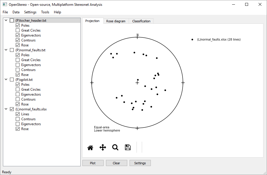
You can also open multiple data files of the same type. Download both normal_faults.xlsx and qplot.txt from the example data and open them using the import plane data (DD) action. Disable the Tocher item and plot the new data:

The normal_faults file contains both the orientation of a plane and a line on each row. As the data set contains no headers, it has no way of detecting which columns contain the attitude for the lines and the planes, so you must provide this information.

The most generic way of opening a data set in OpenStereo is using the Import... action on the file menu. After clicking this and selecting the normal_faults file the following dialog will appear:

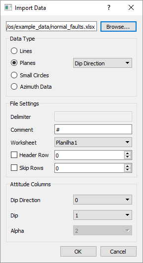
Change the data type to Lines, and the trend and plunge to columns 2 and 3, respectively. Click OK to load the lines, disable the other items and press plot to view the results:

Our project now contains four items, and it’s probably time for some better organization. Right click on any item and select Colapse All to hide the plot options. Rename the items by either using Rename... on the context menu or pressing F2 on your keyboard after selecting an item. After that, you may reorder the items by either clicking and dragging or using the move item actions on the menu. As an example of the results:

There are also some general configurations for the whole project, which can be found by either clicking on the Settings button under the plot or the Project Settings action on the settings menu. This dialog will appear:

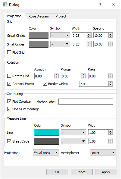
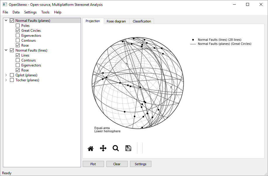
Click on the Plot Grid checkbox to add an equal-area net on your plot. You may also rotate the whole projection by using the rotate grid option. For example, -30.0, 50.0 and 45.0 as azimuth, plunge and rake, respectively. Click Apply to see the results:

You can also see and add some metadata to your project on Project tab on the settings dialog:

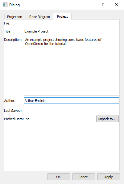
There are two types of OpenStereo project files: regular and packed. They both use the .openstereo extension, and the main difference is that packed projects include the data files inside them, to facilitate sharing projects. Packed projects may be unpacked to a directory using the Unpack to... button on the project tab of the settings dialog.

To finish this tutorial, save the resulting project as a regular one (using either Save or Save as... on the file menu). Regular projects store the relative paths between the .openstereo file and the data files, so you can transport the whole project to different computers by just keeping the same directory structure, as when sharing a folder through Dropbox or a similar service.

If OpenStereo can’t find the data when opening the project, it will ask you for its location. To make this process easier, for each location of these you provide the software will try to find the remaining files relative to both the project file and these given locations.